Demystifying Gradients
- Mathematical Definition and Concepts
- Vanishing and Exploding Gradients
- Mitigations and Solutions
- Best Practice for Model Trainers
- Summary
Gradients are at the core of training LLMs—or any neural network—powering each learning step. You’ve likely heard terms like loss, backpropagation, and optimizers in ML 101, and maybe even vanishing or exploding gradients. But what do these really mean—and how do you handle them in practice?
Whether you’re fine-tuning pre-trained models or training your own from scratch, understanding how gradients behave is essential—it can make or break your training.
This post dives deeper to demystify gradients, exploring:
- The mathematical foundations of gradient computation
- How gradients relate to model design choices like residual connections and normalization
- Practical techniques such as gradient clipping and monitoring gradient behavior during training
Mathematical Definition and Concepts
Gradient
At its core, a gradient is a vector that points in the direction of the steepest ascent of a function. In neural network training, we compute the gradient of the loss function with respect to the model’s parameters. The gradient provides a local map of the loss landscape, indicating how a tiny change in the current parameter state will influence the overall loss.
Figure 1 below illustrates this relationship from two complementary perspectives. The 3D plot visualizes the loss surface. The 2D contour view flattens this landscape into “elevation” lines, making it easier to see how the gradient direction relates to the shape of the landscape. In both views, the gradient is evaluated at a specific parameter point.
Viewed globally, as in Figure 2, the arrows form a gradient field over the loss landscape. The direction of each arrow indicates the steepest ascent of the loss, while its length is proportional to the gradient magnitude—reflecting how rapidly the loss changes locally. A key geometric property is that the gradient is always perpendicular to the contour lines.
During optimization, gradient descent follows the opposite direction of this field. As a result, training typically traces curved trajectories, showing how parameters are updated step by step to reduce the loss.
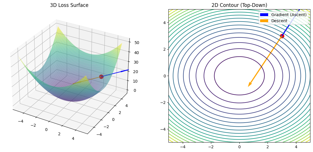
Figure 1: Gradient evaluated at a fixed parameter point on the loss surface (3D vs. 2D).
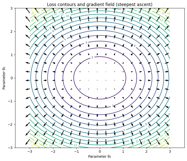
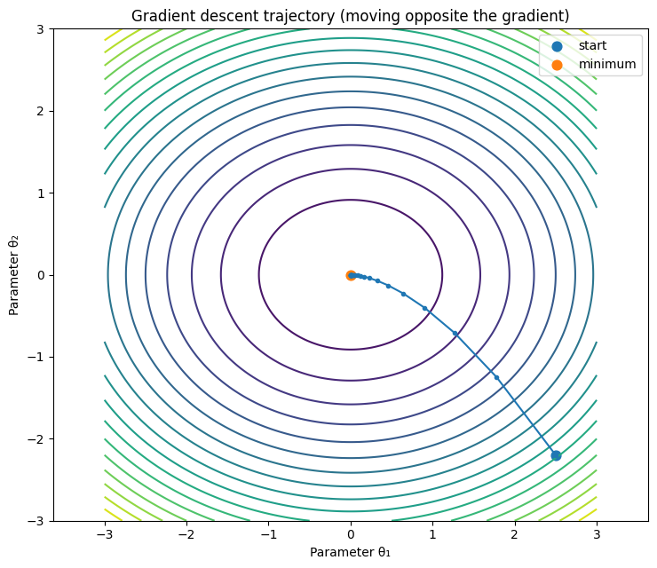
Figure 2: Gradient field (left) and the optimization trajectory (right) of the parameters.
Compute Gradients in Neural Network
Backpropagation is the mechanism that efficiently computes these gradients for all parameters in a neural network. It applies the chain rule from calculus to propagate gradient signals backward from the loss, through each layer, to every weight and bias.
We’ll delve into the analytical results of gradients in a simple network, illustrating how they are sensitive to both input data and network parameters. This sensitivity is crucial to understanding why gradients behave the way they do in deep architectures.
Example Setup: A Simple 2-Layer MLP
To build intuition, consider a very basic Multi-Layer Perceptron (MLP) with:
- Input: $ \mathbf{x} = [x_1, x_2, \dots, x_D] $
- Hidden Layer: 1 neuron with weights $ \mathbf{W}^{(1)} $, bias $ b^{(1)} $
- Output Layer: 1 neuron with weights $ \mathbf{W}^{(2)} $, bias $ b^{(2)} $
- Activation Function: Sigmoid function used in both layers:
\(\sigma(z) = \frac{1}{1 + e^{-z}}\) - Loss Function: Mean Squared Error (MSE)
\(L = \frac{1}{2}(y_{\text{pred}} - y_{\text{true}})^2\)
Forward Pass
-
Hidden Layer Activation: \(a^{(1)} = \sigma(z^{(1)}), \text{where } z^{(1)} = \mathbf{W}^{(1)} \cdot \mathbf{x} + b^{(1)}\)
-
Output: \(y_{\text{pred}} = a^{(2)}= \sigma(z^{(2)}), \text{where } z^{(2)} = \mathbf{W}^{(2)} \cdot a^{(1)} + b^{(2)}\)
-
Loss: \(L = \frac{1}{2}(y_{\text{pred}} - y_{\text{true}})^2\)
Backward Pass: ⛓️ The Chain Rule
The loss depends on the first-layer weights through a chain of intermediate computations:
\[\frac{\partial L}{\partial \mathbf{W}^{(1)}} = \frac{\partial L}{\partial a^{(2)}} \cdot \frac{\partial a^{(2)}}{\partial a^{(1)}} \cdot \frac{\partial a^{(1)}}{\partial \mathbf{W}^{(1)}}\]This sequence illustrates how gradients “flow backward” through the network using the chain rule. Let’s now zoom into each layer and examine the gradient computations in detail.
Output Layer (Layer 2)
We start by calculating the error at the output layer and then its gradients.
- Error at Output ($\delta^{(2)}$). This measures how much the loss changes with respect to the pre-activation ($z^{(2)}$) at the output layer.
\(\delta^{(2)} = \frac{\partial L}{\partial z^{(2)}} = \frac{\partial L}{\partial a^{(2)}} \cdot \frac{\partial a^{(2)}}{\partial z^{(2)}}\)
- Derivative of Loss w.r.t. Output Activation: For MSE, $\frac{\partial L}{\partial a^{(2)}} = (a^{(2)} - y_{\text{true}}) = (y_{\text{pred}} - y_{\text{true}})$
- Derivative of Output Activation w.r.t. Pre-activation: $\frac{\partial a^{(2)}}{\partial z^{(2)}} = \sigma’(z^{(2)})$
- Combining these, the error $\delta^{(2)}$ is:
Now, we use error $\delta^{(2)}$ to find the gradients for the weights and bias of the output layer.
-
Gradient w.r.t. Output Weights ($\mathbf{W}^{(2)}$): \(\frac{\partial L}{\partial \mathbf{W}^{(2)}} = \frac{\partial L}{\partial z^{(2)}} \cdot \frac{\partial z^{(2)}}{\partial \mathbf{W}^{(2)}} = \delta^{(2)} \cdot \mathbf{a}^{(1)}\)
-
Gradient w.r.t. Output Bias ($b^{(2)}$): \(\frac{\partial L}{\partial b^{(2)}} = \frac{\partial L}{\partial z^{(2)}} \cdot \frac{\partial z^{(2)}}{\partial b^{(2)}} = \delta^{(2)} \cdot 1 = \delta^{(2)}\)
Hidden Layer (Layer 1)
Next, we propagate the error backwards to the hidden layer.
- Backpropagated Error ($\delta^{(1)}$) This calculates how much the loss changes with respect to the pre-activation ($\mathbf{z}^{(1)}$) in the hidden layer. It depends on the error from the next layer ($\delta^{(2)}$).
\(\delta^{(1)} = \frac{\partial L}{\partial \mathbf{z}^{(1)}} = \frac{\partial L}{\partial \mathbf{a}^{(1)}} \cdot \frac{\partial \mathbf{a}^{(1)}}{\partial \mathbf{z}^{(1)}}\)
- Derivative of Loss w.r.t. Hidden Activation: This involves propagating the error from the output layer back through the weights: \(\frac{\partial L}{\partial \mathbf{a}^{(1)}} = \mathbf{W}^{(2)T} \delta^{(2)}\)
- Derivative of Hidden Activation w.r.t. Pre-activation: $\frac{\partial \mathbf{a}^{(1)}}{\partial \mathbf{z}^{(1)}} = \sigma’(\mathbf{z}^{(1)})$
- Combining these, the error $\delta^{(1)}$ for the hidden layer is:
Finally, we use $\delta^{(1)}$ to find the gradients for the weights and bias of the hidden layer.
-
Gradient w.r.t. Hidden Weights ($\mathbf{W}^{(1)}$): \(\frac{\partial L}{\partial \mathbf{W}^{(1)}} = \frac{\partial L}{\partial \mathbf{z}^{(1)}} \cdot \frac{\partial \mathbf{z}^{(1)}}{\partial \mathbf{W}^{(1)}} = \delta^{(1)} \mathbf{x}^T\) (This is the outer product of the error $\delta^{(1)}$ and the input $\mathbf{x}$.)
-
Gradient w.r.t. Hidden Bias ($b^{(1)}$): \(\frac{\partial L}{\partial b^{(1)}} = \frac{\partial L}{\partial \mathbf{z}^{(1)}} \cdot \frac{\partial \mathbf{z}^{(1)}}{\partial b^{(1)}} = \delta^{(1)}\)
Vanishing and Exploding Gradients
The Core Problem: Products of Weights and Derivatives.
In our backpropagation derivation, the error term for a layer, $\delta^{(l)}$, is calculated by propagating the error from the subsequent layer, involving a product with that layer’s weights and the derivative of the current layer’s activation function:
\[\delta^{(l)} = (\mathbf{W}^{(l+1)T} \delta^{(l+1)}) \odot \sigma'(\mathbf{z}^{(l)})\]When we calculate the gradient for the weights of an early layer, say $\mathbf{W}^{(1)}$, this process involves a chain of multiplications through all subsequent layers. If we had more layers, say up to layer $N$, the error $\delta^{(1)}$ would effectively look something like this in a simplified chain rule expansion (ignoring specific matrix operations for clarity):
\[\delta^{(1)} \propto \delta^{(N)} \cdot (\mathbf{W}^{(N)}) \cdot \sigma'(\mathbf{z}^{(N-1)}) \cdot (\mathbf{W}^{(N-1)}) \cdot \sigma'(\mathbf{z}^{(N-2)}) \cdots (\mathbf{W}^{(2)}) \cdot \sigma'(\mathbf{z}^{(1)})\]This expression highlights a critical point > the error signal for earlier layers is a product of many terms, specifically the weights ($\mathbf{W}$) and the derivatives of the activation functions ($\sigma’(\mathbf{z})$) from all subsequent layers.
In addition, > the gradient of the loss function with respect to the hidden weights $W^{(l)}$ is the product of the error term and the activation from the previous layer (or input):
\[\frac{\partial \mathcal{L}}{\partial \mathbf{W}^{(l)}} = \delta^{(l)} (a^{(l-1)})^T, \text{where } a^{(0)} = \mathbf{x}\]Vanishing Gradients
If activation derivatives and/or weights have magnitudes consistently less than 1 (e.g., $\Vert\sigma’(z)\Vert < 1, \Vert\mathbf{W}\Vert < 1$), their repeated multiplication during backpropagation causes gradient magnitudes to decay exponentially with network depth.
Impact: Gradients for parameters in earlier layers become extremely small, often approaching numerical zero. As a result, updates to these parameters are negligible, causing early layers to learn very slowly or effectively stop learning altogether.
Exploding Gradients
Conversely, if weights or activation derivatives have magnitudes consistently greater than 1 (e.g., $\Vert\mathbf{W}\Vert > 1$), the repeated multiplication causes gradient magnitudes to grow exponentially as it propagates toward the input layer during backpropagation.
Impact: Gradients become excessively large, leading to massive updates to the network parameters. This causes the optimization process to become unstable, manifesting as oscillatory loss curves. In severe cases, this leads to numerical overflow (NaNs), causing the model to diverge and training to fail completely.
Contributing Factors
From the analysis above, both vanishing and exploding gradients are exacerbated by several factors in deep networks:
-
Number of Layers (Network Depth): The deeper the network, the more multiplications are involved in the backpropagation chain, magnifying the effect of both small and large values.
- Activation Function Saturation:
- Sigmoid and Tanh: These functions are highly susceptible to vanishing gradients when they enter “saturation regions.” In these regions, the input values are very large or very small, causing the derivatives to approach zero.
- ReLU: Unlike Sigmoid, the ReLU derivative is either 0 or 1. Here, “vanishing” occurs when neurons stay “off” (derivative is 0). This is known as the “Dying ReLU” problem.
- Weight Initialization:
- Too Small: Can push activation outputs toward the flat regions (near 0 for Tanh/Sigmoid), leading to vanishing gradients;
- Too Large: Can cause activations to become extreme, leading to saturation in Sigmoid/Tanh or direct amplification (exploding) in ReLU.
- Nature of Data:
- Scaling: Poorly scaled input data can lead to extreme pre-activation values, pushing neurons into saturated regions.
- Outliers and Noise: A “bad batch” containing extreme outliers can produce a massive error signal, createing an explosive update.
Visualization
- Vanishing Gradients (Sigmoid + Small Initialization). The left figure illustrates the vanishing gradient phenomenon using sigmoid activations and small weight initialization. As gradients are backpropagated toward earlier layers, they are repeatedly multiplied by sigmoid derivatives and weight matrices whose magnitudes are less than one. Each step slightly shrinks the signal, and over many layers this compounding effect causes the gradient to fade away. On a logarithmic scale, this appears as a smooth, straight downward line: every layer closer to the input receives a consistently smaller update. In practice, this means early layers barely learn, even though the network continues to update parameters near the output.
- Exploding Gradients (ReLU + Large Initialization). Here, large weights amplify the backpropagated gradient. ReLU activations either pass gradients through unchanged or block them entirely, and each weight matrix amplifies different directions by different amounts. As a result, gradient magnitudes surge and collapse unpredictably from layer to layer, producing sharp spikes and drops on the log scale. This erratic behavior reflects an unstable optimization process, where parameter updates can become excessively large, causing oscillations.
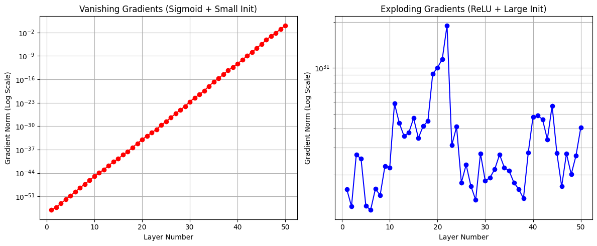
Figure 3. Gradient norm per layer (Vanishing vs. Exploding).
Mitigations and Solutions
Mitigation strategies therefore fall into three broad categories:
- Local fixes: Techniques that act directly on the multiplicative factors in backpropagation by controlling their magnitude.
- Activation functions: Shape activation derivatives.
- Weight initialization: Regulate the scale of weight matrices.
- Gradient clipping: Prevent extreme gradient updates during optimization.
- Structural fixes: Techniques that modify how gradients flow through the network.
- Residual connections: Shorten effective gradient paths.
- Normalization layers: Stabilize activation and gradient distributions.
- Data-Centric Solutions: Practices that improve gradient behavior by conditioning the input data before learning begins.
Let’s start with the simple direct local fixes before moving on to structural, architectural solutions.
Activation Functions
Activation functions directly influence the magnitude of the derivative $\sigma’(z)$, which appears in every layer’s error term during backpropagation. As a result, activation choice plays a critical role in preserving gradient signal as depth increases.
-
Prefer non-saturating activations. Modern architectures typically favor activations that avoid saturation, such as ReLU and its variants (e.g., Leaky ReLU) or smooth alternatives like GELU. These functions preserve non-trivial derivatives over a wide range of inputs, allowing gradients to propagate backward without rapidly shrinking.
-
Mitigate inactive regions. Standard ReLU is susceptible to the “Dying ReLU” problem, where neurons output zero for all inputs, effectively halting gradient flow. Variants like Leaky ReLU introduce a small slope (e.g., $0.01$) for negative inputs, ensuring that even “off” neurons maintain a non-zero gradient and can eventually recover during training.
To make these ideas concrete, we visualize these behaviors in Figure 4. Note how the derivatives of Sigmoid and Tanh approach zero quickly, while ReLU-based derivatives maintain constant magnitudes, providing a “highway” for the gradient.
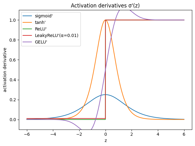
Figure 4. Activation derivatives.
- Pairing with initialization. Activation choice should be paired with an appropriate initialization scheme (coming up next) to maintain stable signal propagation.
Weight initialization
Initialization sets the starting conditions for gradient flow. It does not solve vanishing or exploding gradients, but it prevents the network from starting in a pathological regime. Take a simplified pre-activation $\mathbf{z}^{(l)} = \mathbf{W}^{(l)} \mathbf{a}^{(l-1)}$, its variance depends on $\mathrm{Var}(\mathbf{W}^{(l)})$. Its scaling, however, depends on how the activation function transforms its input.
- Xavier (Glorot) initialization is designed for symmetric activations like Sigmoid and Tanh activations and scales initial weights based on the number of input and output units.
Around the center of the derivative curve, the sigmoid and tanh function are approximately linear. Xavier initialization aims to keep the “pre-activation” values ($z$) within this central region (roughly $-2<z<2$ for sigmoid), allowing signals to pass through each layer without excessive attenuation. By depending on both fan_in and fan_out, Xavier initialization balances the scale of forward activations and backward gradients, keeping their variances roughly constant in expectation at initialization.
- Kaiming (He) initialization is designed for ReLU-based activations, which zero out negative inputs. For zero-mean inputs, this means that roughly half of the activations are zero in expectation, reducing the variance of the signal by about a factor of two. To compensate, Kaiming initialization scales weights using only the number of input units and increases the variance accordingly:
This scaling preserves the magnitude of forward activations and is typically sufficient to keep backward gradients stable at initialization for ReLU-based networks.
Figure 5 demonstrates the impact of these strategies. We plot the gradient norm of each layer’s weights after a single backward pass. This allows us to directly observe how different combinations of activations and initialization influence gradient propagation across depth.
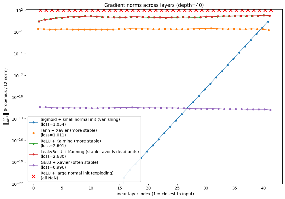
Figure 5. Gradient Norm under different activations + initialization
Gradient clipping
Gradient clipping limits the magnitude of gradients after they are computed but before parameters are Gradient clipping limits the magnitude of gradients after they are computed via backpropagation but before parameters are updated. It does not address the root cause of exploding gradients. Instead, it acts as a safety mechanism that prevents catastrophic parameter updates caused by rare but extreme gradient values (for example, when an occasional batch produces an unusually large error signal). Two clipping strategies are commonly used:
- Clipping by value. Each individual gradient element is independently clamped to lie within a fixed range. For example, the following code clamps every gradient component to the interval $[−1.0, 1.0]$. This approach directly limits extreme gradient components but may distort the overall gradient direction.
torch.nn.utils.clip_grad_value_(model.parameters(), clip_value=1.0)
- Clipping by global norm. Clipping by global norm rescales all parameter gradients by the same factor whenever their combined norm exceeds a specified threshold. In the following code, if the total gradient norm exceeds
max_norm($1.0$), all gradients are scaled down proportionally so that the global norm equalsmax_norm.total_normreturns the total norm before clipping.
total_norm = torch.nn.utils.clip_grad_norm_(model.parameters(), max_norm=1.0)
In comparison with Clipping by value, Clipping by global norm preserves the direction of the gradient vector while only reducing its magnitude, since the relative proportions between gradient elements remain unchanged. As a result, it does not alter the descent direction chosen by the optimizer, but only shortens the step taken in that direction, as shown in Figure 6. From an optimization perspective, this acts as a temporary reduction in the effective learning rate during unstable steps.
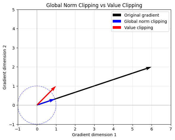
Figure 6. Global gradient norm clipping vs Value clipping.
In pytorch, you can apply gradient clipping immediately after loss.backward() and before optimizer.step(). In practice, you can log total_norm. By capturing the norm before it is clipped, we can monitor the stability of the training process.
loss.backward()
total_norm = torch.nn.utils.clip_grad_norm_(
    model.parameters(),
    max_norm=1.0
)
print("Grad norm before clipping:", total_norm.item())
optimizer.step()
Residual connections
We now shift from local techniques to architectural design choices. One effective way to reduce vanishing gradients in very deep networks is to avoid forcing gradients to propagate through too many consecutive layers.
Residual connections mitigate this by introducing skip connections that allow gradients to flow directly across layers. Concretely, a residual block preserves the identity input $x$ and learns a residual function $F(x)$, which is added to the input:
\[y = x + F(x)\]This design has a direct and important consequence for backpropagation. Differentiating with respect to $x$ gives:
\[\frac{\partial y}{\partial x} = I + \frac{\partial F(x)}{\partial x}\]The identity term $I$ ensures that, regardless of the behavior of the residual branch $F(x)$, there is always a gradient path that does not vanish through repeated multiplications. Even if $\frac{\partial F(x)}{\partial x}$ becomes small due to activation saturation or poor conditioning, the gradient can still flow through the identity connection. Residual connections thus provide a “shortcut” for gradients, rather than forcing information to pass through a long, fragile chain of transformations.
Residual connections are a fundamental building block in deep neural networks, most notably ResNets and Transformers (which large language models are based on), because they make very deep networks significantly easier to optimize.
Normalization layers
Normalization layers aim to keep activations within a stable range during training. By regularizing the distribution of activations, normalization reduces sensitivity to weight initialization, learning rate, and input scale, and improves the conditioning of both forward and backward passes. In deep networks, normalization is especially important because it helps prevent activations from drifting into regimes where gradients vanish or explode. Two commonly used normalization techniques are:
- Batch Normalization
- Layer Normalization
There are many excellent resources that cover this topic in depth (for example, the article from Pinecone: Batch and Layer Normalization). Here, we provide a brief overview and focus specifically on how these methods help stabilize gradient flow.
Batch Normalization
Batch Normalization (BatchNorm) normalizes activations across the batch dimension for each feature. It uses batch-level statistics – the mean and standard deviation computed from the current mini-batch. BatchNorm is highly effective in convolutional and feed-forward networks and has been a key enabler of very deep CNNs.
Batch Normalization has two important limitations: * When the batch size is small, the sample mean and sample standard deviation are not representative enough of the actual distribution, leading to unstable or degraded learning. * Batch normalization is less suited for sequence models, which may have sequences of potentially different lengths.
Layer Normalization
Layer Normalization (LayerNorm) normalizes activations across the feature dimensions within each individual sample. Unlike BatchNorm, LayerNorm does not rely on batch statistics. Normalization is performed independently for each sample, making it robust to small batch sizes and variable-length inputs.
LayerNorm provides per-token normalization, which is critical for sequence modeling and autoregressive generation.
In a sequence model, given an activation tensor of shape $(B, T, d)$ (batch size $B$, sequence length $T$, hidden dimension $d$), LayerNorm operates on each token representation $\mathbf{x}_{b,t} \in \mathbb{R}^d$ independently. For a single token representation $\mathbf{x}$, LayerNorm applies the following transformation:
\[\mathrm{LayerNorm}(\mathbf{x}) = \gamma \odot \frac{\mathbf{x} - \mu}{\sqrt{\sigma^2 + \epsilon}} + \beta\]where the statistics are computed across the feature dimension of that token:
\[\mu = \frac{1}{d} \sum_{i=1}^d x_i, \quad \sigma^2 = \frac{1}{d} \sum_{i=1}^d (x_i - \mu)^2\]No statistics are computed across tokens in the sequence or across the batch. Note that LayerNorm changes the numerical scale (absolute magnitude) of a token’s representation, not its semantic meaning (relative pattern of features within). In addition, LayerNorm includes learnable parameters that restore representational flexibility:
- $\gamma$: feature-wise scaling
- $\beta$: feature-wise shifting
As a result, LayerNorm does not constrain representations to remain at zero mean and unit variance throughout training. Instead, it provides a stable numerical starting point, while allowing the network to learn task-specific rescaling and shifting of features as needed.
In an autoregressive model, the context grows with every new token generated, and tokens are processed sequentially rather than in large, fixed batches. LayerNorm is critical because it normalizes each token’s representation independently of other tokens in the sequence or batch. This ensures that each token’s hidden state remains numerically well-conditioned as it passes through many layers, even as the sequence grows longer.
This property makes LayerNorm the standard choice in Transformer architectures for large language models (LLM). By ensuring that each token’s representation remains well-conditioned, LayerNorm helps maintain stable gradients throughout very deep Transformer stacks.
RMSNorm
RMSNorm(Root Mean Square Normalization) is motivated by the observation that the re-centering step of LayerNorm (subtracting the mean $\mu$) is computationally expensive and less important for stability than the re-scaling property. By removing the mean calculation and the additive bias term. RMSNorm therefore removes the mean subtraction and focuses solely on normalizing the magnitude of the activation vector via its root mean square:
\[\mathrm{RMSNorm}(\mathbf{x}) = \gamma \odot \frac{\mathbf{x}}{\sqrt{\frac{1}{d} \sum_{i=1}^d x_i^2 + \epsilon}}\]Unlike LayerNorm, RMSNorm drops the additive bias term ($\beta$) entirely and learns only a feature-wise scaling parameter $\gamma$. By eliminating the mean computation and subtraction, RMSNorm reduces both computational overhead and parameter count, leading to improved hardware efficiency and better utilization on modern accelerators. From an optimization perspective, RMSNorm also simplifies backpropagation. Its gradients are slightly cheaper to compute than those of LayerNorm, resulting in marginally faster backward passes and reduced memory pressure during training.
Empirically, removing the mean has been shown to have little to no negative impact on model quality. RMSNorm provides similarly well-conditioned inputs to subsequent layers by keeping activation magnitudes in a predictable range. As a result, it is widely adopted in recent LLM models (PaLM / Chinchilla, Mistral / Mixtral, LLaMA (1/2/3), Qwen, DeepSeek).
Interaction of Normalization with Residuals
In Transformer architectures, normalization layers and residual connections are tightly coupled. A critical architectural design choice is where normalization is applied relative to the residual connection. This leads to two common variants: Post-Normalization and Pre-Normalization.
Post-Normalization
In the original Transformer architecture, Post-Normalization(Post-LN) is used: normalization is applied after the residual connection.
\[\text{output} = \mathrm{LayerNorm}(x + F(x))\]Here, $F(x)$ represents the main operation (e.g., self-attention or a feed-forward block).
While this design preserves the residual structure, applying normalization after the addition modifies the identity path itself. The signal $x$, intended to serve as a clean shortcut for gradients, is immediately rescaled and shifted by LayerNorm. As a result, the identity path is no longer pristine and gradients must still pass through the normalization operation.
The interaction between residual connections and normalization placement has been studied in detail by Xiong et al. in On Layer Normalization in the Transformer Architecture. Figure 7 (adopted from the paper) illustrates the structural difference between Post-Normalization and Pre-Normalization Transformer blocks.
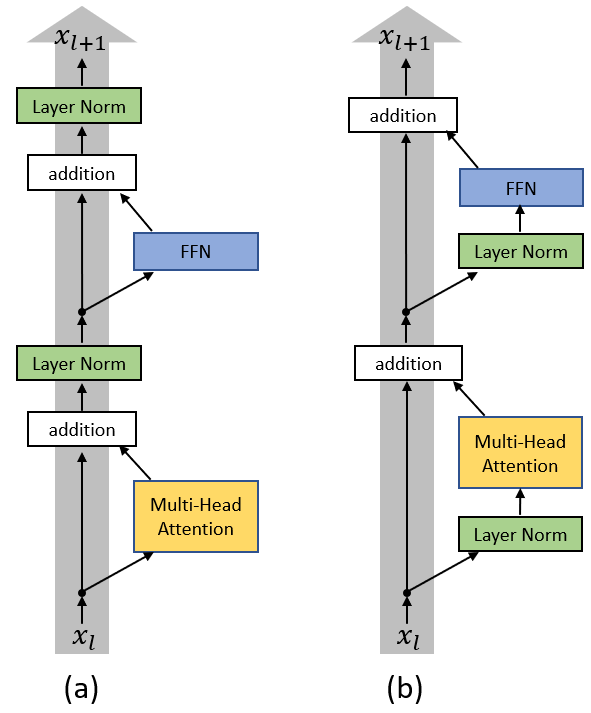
Figure 7. Comparison of Post-Normalization (a) and Pre-Normalization (b) Transformer architectures.
Pre-Normalization
In Pre-Normalization (Pre-LN), normalization is applied before the main operation, while the residual connection adds back the original input unchanged:
\[\text{output} = x + F(\mathrm{LayerNorm}(x))\]This design preserves a true identity path for the residual connection, enables larger learning rates, fewer gradient spikes, leading to improved training stability. As a result, though the original transformer and BERT use Post-LN, Pre-LN has become the de facto standard in modern Transformer architectures (GPT-2 / GPT-3, LLaMA (1/2/3), PaLM / Chinchilla, Mistral / Mixtral, Qwen, DeepSeek).
Beyond Pre-LN: Double Normalization
While Pre-LN is the current standard, a new design space is emerging. Recent LLM architectures like Gemma 2, Grok, and OLMo 2 have begun experimenting with Double Normalization. In these designs, Pre-LN remains inside each block to stabilize the inputs to Attention and FFN layers, while an additional normalization layer is placed at the end of the block. It avoids the drawbacks of the classic Post-LN by preserving a clean residual identity path while still applying extra normalization at carefully chosen points.
Further Reading
For a more comprehensive discussion of Transformer architecture choices, including normalization placement, residual design, and stability considerations, I would recommend CS336: Language Modeling from Scratch (2025), Lecture 3: Architectures & Hyperparameters.
Data Cleaning
Recall the gradient of the loss with respect to the first-layer weights:
\[\frac{\partial \mathcal{L}}{\partial \mathbf{W}^{(1)}} = \delta^{(1)} \mathbf{x}^T\]If the input $\mathbf{x}$ is poorly conditioned, the gradient is compromised from the very first layer.
-
Feature Scaling. When input features have vastly different ranges (e.g., one feature lies in the range $[0, 1]$ while another lies in $[0, 1000]$), the loss landscape becomes highly elongated. Gradients corresponding to different dimensions then differ drastically in magnitude, making optimization sensitive to learning rate. In traditional ML, it is a common practice to standardize inputs to zero mean and unit variance ensures that signals entering the network are comparably scaled, reducing the risk of early-layer saturation and improving gradient conditioning. In contrast, LLMs do not operate on raw numeric features; token embeddings and pervasive normalization layers (e.g., LayerNorm or RMSNorm) implicitly control scale throughout the network. As a result, explicit feature scaling is typically unnecessary for LLM training itself, but remains important at system boundaries, such as reward modeling or when integrating external numerical signals.
-
Handling Outliers and “Bad Batches”. In traditional machine learning trained on numeric inputs, a single extreme data point can generate a disproportionately large error term. In LLM training, a single ‘bad’ batch (garbled text, nonsensical sequences, extreme outliers) can trigger a gradient spike, causing overflow and resulting in NaN values that propagate through the entire network, killing the training process and forcing a costly rollback to a previous checkpoint. Because LLMs are often trained with very large batch sizes (millions of tokens per step), the averaged gradient for that entire step becomes corrupted if even a small portion of the data is nonsensical. Therefore, careful data cleaning and robust preprocessing are a prerequisite for stable training at scale.
Best Practice for Model Trainers
Understanding why gradients vanish or explode is only half the story. In practice, stable training requires being able to observe, diagnose, and respond to gradient behavior during training. This section focuses on concrete techniques model trainers can use to monitor and control gradients in real systems, from small PyTorch experiments to large-scale LLM training.
Accessing Gradients in PyTorch
In PyTorch, every parameter that has requires_grad=True will store its gradient in the .grad attribute after loss.backward() is called.
# Example in PyTorch (conceptual)
import torch
import torch.nn as nn

# Define a simple model
model = nn.Linear(10, 1)
loss_fn = nn.MSELoss()
optimizer = torch.optim.SGD(model.parameters(), lr=0.01)

# Dummy data
x = torch.randn(1, 10)
y_true = torch.randn(1, 1)

# Forward pass
y_pred = model(x)
loss = loss_fn(y_pred, y_true)

# Backward pass to compute gradients
loss.backward()

# Access gradients
for name, param in model.named_parameters():
    if param.grad is not None:
        grad_norm = param.grad.norm().item()
        grad_max = param.grad.max().item()

        # Check for the dreaded NaN
        if torch.isnan(param.grad).any():
            print(f"⚠️ Exploded! NaN detected in {name}")

        print(f"Layer: {name} | Norm: {grad_norm:.4f} | Max: {grad_max:.4f}")
You can get the following output
Layer: weight | Norm: 8.5318 | Max: 4.9751
Layer: bias | Norm: 2.6719 | Max: -2.6719
Monitor Gradients During Training
Most professional teams use tools like Weights & Biases (W&B) to visualize gradient health. While the loss curve and gradient curves both provide information about stability, they represent different perspectives of the training process:
-
The Loss Curve (Symptoms): The loss curve tells you if the model is converging and acts as a high-level indicator of stability. A “jagged” loss curve with frequent spikes suggests training is struggling with learning rate or data quality. A sudden vertical jump in loss (a “loss spike”) is the most common visible symptom of training instability.
-
The Gradient Curves (Root Cause): Gradients provide a more direct prognostic signal. By monitoring gradient norms, it is often possible to detect instability before it manifests in the loss. If gradient norms begin to grow rapidly or trend upward exponentially, a loss spike or divergence is often imminent.
Key Gradient Signals to Watch
- Global Gradient Norm: A single scalar summarizing the overall magnitude of gradients across all parameters. This is often the most useful first-line stability signal. A healthy run shows a stable or slowly decaying norm, while sudden spikes frequently precede training collapse.
- Layer-wise Norms: Inspecting gradients per layer is one of the most effective ways to diagnose architectural issues. If gradients in early layers are consistently much smaller than those in later layers, this strongly suggests vanishing gradients.
- Gradient Distributions (Histograms): Visualizing the distribution of gradient values over time can reveal subtle pathologies such as heavy tails, extreme outliers, or mass accumulation near zero—patterns that scalar metrics may miss.
- Weight-to-Update Ratio: A practical diagnostic is the ratio between the parameter update magnitude and the parameter magnitude: $\Vert\Delta W\Vert / \Vert W\Vert$. Values on the order of $10^{-3}$ are typically reasonable. Consistently larger values indicate an overly aggressive learning rate; much smaller values suggest the model is barely learning.
Summarized in the table below, these gradient-level diagnostics provide a more direct and actionable view of training health than the loss curve alone, enabling earlier intervention and more targeted mitigation strategies.
Common Warning Signs and Mitigations
| Warning Sign | Likely Issue | Typical Mitigation |
|---|---|---|
| Sudden spikes in global gradient norm | Impending numerical instability | Lower learning rate; tighten gradient clipping |
| Gradients become NaN or Inf | Overflow or unstable updates | Enable clipping; Checking training precision change; reduce learning rate |
| Near-zero gradients in early layers | Vanishing gradients | Check residual connections; verify normalization placement |
| Instability tied to specific data batch | Pathological batches or data issues | Improve data filtering; adjust batching strategy |
Leveraging Modern LLM training frameworks
Modern LLM training frameworks (e.g., Accelerate, DeepSpeed, FSDP, Megatron-LM) all expose hooks for gradient monitoring. For example, Megatron-LM logs the grad_norm by default in its training loops. While implementations vary, they follow a unified operational logic: gradients are accumulated across micro-batches, norms are calculated at global step boundaries, and Gradient Clipping and logging are executed immediately before parameter updates. Understanding these mechanics is essential for interpreting training logs. By mastering these tools, developers can move from simply observing training failures to proactively debugging them at scale. The specific implementation details of large-scale LLM training framework deserve a deep dive of their own. Stay tuned for a future post on that topic.
Summary
Architectural choices like residual connections and normalization lay the foundation for stable gradient flow, but monitoring and controlling gradients is what keeps large model training on track. Effective trainers treat gradient inspection as a first-class diagnostic tool. Just like life is a continuous hill-climbing journey towards your goals, gradients represent each strategic step. Happy gradient ascending in 2026!