Reflections on Richard Sutton's Interview: Part II — Goal and Acting
- Sutton’s View: Intelligence Requires a Goal
- Two Approaches to RL
- LLMs as Policies
- From Behavior Cloning to Reinforcement Learning
- Open Reflections
- Closing Thought
Understanding describes the world; goals decide what to do in it.
In Part I, I discussed world model — what is it, why it is central to intelligence, how it can be built, how LLMs build such understanding, and where that understanding falls short. In this second part, I turn to the other half of intelligence: acting toward a goal.
Sutton’s View: Intelligence Requires a Goal
As Richard Sutton reminds us of John McCarthy’s classic definition:
“Intelligence is the computational part of the ability to achieve goals.” — John McCarthy
Let’s begin again with the simplest form for expressing this objective. In reinforcement learning (RL), acting toward a goal is formalized through the Markov Decision Process (MDP).
Recall that the world model (or dynamics model) describes how the environment changes and how rewards are generated based on the agent’s actions. This model provides the underlying components of the MDP:
\[\begin{aligned} s_t &= g(o_t) && \text{(state inference)} \\ s_{t+1} &\sim P(s_{t+1} \mid s_t, a_t) && \text{(stochastic transition)} \\ r_t &= r(s_t, a_t) && \text{(reward model)} \\ o_t &\sim P(o_t \mid s_t) && \text{(observation generation)} \end{aligned}\]While the dynamics model tells us what will happen (the mechanics of the world), the objective tells us what matters (the agent’s goal). We need a mathematical expression that formalizes this goal — one that captures intelligence as the ability to pursue desirable outcomes over time. This objective is formally defined as the expected cumulative discounted reward, or return:
Objective
This objective is defined as the expected cumulative discounted reward, or return:
\[J = \mathbb{E}\!\left[\sum_t \gamma^t r_t\right]\]where:
- $\mathbb{E}$ denotes the expected value of the reward sequence under the model’s behavior.
- $\gamma \in [0,1]$ is the discount factor, ensuring that rewards received sooner are valued more highly than those received later.
- $T$ is the time horizon, which may be finite or infinite.
Policy
To act toward a goal, the agent needs a rule to decide what to do in order to optimize its reward. This rule is called the policy. Concretely, a policy $\pi(a\mid s)$ is a mapping from states to actions that dictates the agent’s behavior at every time step. It defines how the agent behaves, given what it currently knows about the world.
The goal in reinforcement learning is to find the optimal policy — the one that maximizes the expected cumulative discounted reward (or return) over time.
In most cases, the policy is stochastic, meaning that the agent selects actions according to a probability distribution conditioned on the current state:
\[a_t \sim \pi(a_t \mid s_t)\]This allows for exploration — the ability to sample different actions and discover better strategies over time.
Formally, the optimization objective can be expressed as:
\[J(\pi) = \mathbb{E}_{\tau \sim \pi} \left[ \sum_{t=0}^{T} \gamma^t r_t \right]\]where $\tau = (s_0, a_0, s_1, a_1, \ldots)$ denotes a trajectory sampled according to the policy $\pi$. The goal of learning is to find the policy $\pi^*$ that maximizes this expected return:
\[\pi^* = \arg\max_{\pi} J(\pi)\]Two Approaches to RL
At a high level, reinforcement learning methods fall into two broad categories, depending on whether the agent has access to (or learns) a dynamics model. The diagram below (from OpenAI Spinning Up) summarizes these families of RL algorithms:

-
Model-based RL Model-based methods use an explicit world model to simulate and plan future actions before execution. The key advantage is foresight — the ability to “think ahead,” evaluate the consequences of possible actions, and select the best one before acting.
By using its model to plan, the agent can distill the results of this reasoning process into a learned policy.The main challenge is the availability of the dynamics (world) model. An imperfect model can mislead the agent into optimizing for its own errors — performing well within the learned model but failing in the real world.
-
Model-free RL Model-free methods, by contrast, does not need an explicit world model, rather, it learns directly from experience. Instead of simulating possible futures, the agent interacts with the environment, receives rewards, and gradually adjusts its behavior based on observed outcomes.
This family includes two major subcategories — value-based and policy-based approaches.
Value-Based Approach
Value-based methods estimate the long-term return of each state or action using a value function $V(s)$ or an action-value function (or Q-function) $Q(s, a)$. These functions predict how good it is to be in a certain state or to take a certain action, in terms of future rewards. The value function is one of the four fundamental components of Sutton’s “base common model” of the RL agent.
This estimation connects short-term actions to long-term goals — a mechanism for learning from sparse rewards that occur far in the future. Sutton’s startup analogy captures this idea well: Imagine an entrepreneur working toward a long-term goal: the reward may arrive once in ten years — the “exit” moment when the startup succeeds. To stay motivated and effective, humans construct intermediate signals of progress: milestones, customer feedback, or product growth. Each small improvement updates the belief that the long-term goal is achievable, reinforcing the behaviors that contribute to it.
In RL, the value function serves this same purpose. When an agent achieves a local success it updates its estimate of eventual victory. That increase in expected value immediately reinforces the move that led to it. This mechanism, known as temporal-difference (TD) learning, allows the agent to convert distant goals into immediate learning signals.
In essence, the value function transforms long-term objectives into tangible, auxiliary predictive rewards that drive learning in the moment.
Policy-Based Approach
The policy is another fundamental component of the RL agent based on Sutton’s “base common model” — the part that determines how it acts. Policy-based methods (also called policy optimization) take a different route from value-based ones. Rather than estimating value functions first, they directly optimize the policy parameters to improve expected performance.
A common technique, known as the policy gradient method, adjusts the policy parameters in proportion to the goodness of outcomes. Intuitively, actions that lead to higher returns are made more likely, while less successful actions are suppressed.
Formally, the policy gradient can be written as:
\[\nabla_\theta J(\pi_\theta) = \mathbb{E}\!\left[\nabla_\theta \log \pi_\theta(a|s) \, Q^\pi(s,a)\right]\]This equation expresses a simple but profound idea: the gradient of performance depends on how likely an action is under the current policy and how valuable that action turns out to be. By following this gradient, the agent continually improves its behavior through experience.
Sutton summarized this intuitively in his interview:
“You act, you see what happens, and you change your behavior accordingly — not because someone told you what to do, but because the world responded.”
This captures the essence of policy-based RL — intelligence as the art of adjustment to feedback.
LLMs as Policies
Large Language Models (LLMs) can be viewed as policy models that map a given context (prompt) to a distribution over next-token actions. Sampling from the model corresponds to executing a stochastic policy $\pi_\theta(a_t \mid s_t)$, where:
- $s_t$: the current input sequence,
- $a_t$: the token selected at time step $t$,
- $\theta$: the model parameters.
And language generation can be expressed as a Markov Decision Process (MDP), where
- Transition is deterministic: $s_{t+1} = s_t \circ a_t$,
- Reward $r$ is a scalar value provided after sequence generation.
To understand how this policy is learned — and how it differs from Sutton’s view — we must ask: Does it have a goal? And if so, what is that goal? Let’s look at how large language models are trained to seek an answer.
From Behavior Cloning to Reinforcement Learning
LLMs undergo a multi-stage training process as Pre-Training and Post-Training, which usually includes Supervised Fine-Tuning (SFT) and Reinforcement Learning with various types of rewards Human Feedback (RLHF), Verifiable Reward (RLVF), etc.
Pretraining and SFT: Policy from Imitation
In pretraining, the policy is optimized for next-token prediction from pretraining data — learning to imitate human linguistic behavior. This imitation-based paradigm effectively mirrors human language distributions rather than optimizing for outcomes. The model’s capability is limited by the quality and diversity of its training data. Without goal-driven correction, any flaws or biases in human data are inherited.
In SFT, the policy is trained directly on human demonstrations. Given an input context $s_t$, the model learns to predict the next token $a_t$ that aligns with a human-provided reference output. Formally, the objective minimizes the negative log-likelihood of the target sequence:
\[\mathcal{L}_{\text{SFT}} = - \sum_t \log \pi_\theta(a_t^{*} \mid s_t)\]Here, $a_t^{\ast}$ represents the human-annotated “correct” token at each step.
Through this process, the model learns to imitate expert behavior — optimizing per-token likelihood given the context, rather than optimizing for task-specific rewards. SFT refines the base model to follow human intent more reliably, but it remains fundamentally imitation-based. As a result, SFT has the following limitations:
- Performance Ceiling: The model is constrained by the quality of its demonstrations. When the demonstrations are suboptimal, the resulting policy cannot surpass them and often inherits their flaws.
- Limited Generalization: Unable to adapt to unseen context. When the model deviates from the demonstrated trajectory and encounters out-of-distribution states, it can not recover.
- High Data Costs: Curating large-scale, high-quality human demonstration data is expensive and slow.
Reinforcement Learning in Post-Training: Policy with a Goal
Post-training introduces explicit goals through reinforcement learning.
- In RLHF (Reinforcement Learning from Human Feedback), reward model is a learned neural network reflecting human preference.
- In RLVR (Verifiable Reward), rewards are derived from objective task success signals — such as solving a math problem or producing functionally correct code.
- In RLAIF (AI Feedback), the reward model is trained from preferences generated by a stronger or more aligned AI system rather than human annotators.
These techniques transform LLMs from passive imitators into systems that optimize for defined reward/outcomes.
Open Reflections
Is RL in Post-Training Enough?
On the road to scaling RL, it’s pivotal to preserve exploration so the policy can keep finding novel trajectories rather than over-exploiting what already works. This is the classical exploration–exploitation dilemma in RL. For LLMs, this trade-off appears at every generation step: each token is an action sampled from the current model’s policy, so “exploration” is realized by sampling diversity. The diversity of this sampling is commonly quantified by policy entropy; higher entropy generally promotes broader exploration, while lower entropy tends to premature convergence.
In practice, RL for LLMs operates under two major constraints:
- Policy-entropy decay. During RL fine-tuning of LLMs, policy entropy often declines over training—sometimes sharply if without explicit entropy or diversity controls. This makes the policy increasingly deterministic and reducing its ability to discover alternate paths. This reduction in exploration is frequently associated with performance plateaus. Once the policy’s capacity for probabilistic exploration is exhausted, the model’s potential to improve through additional training or scaling becomes marginal.

Figure source: “The entropy mechanism of reinforcement learning for reasoning language models.” arXiv:2505.22617.
- KL Divergence Regularization
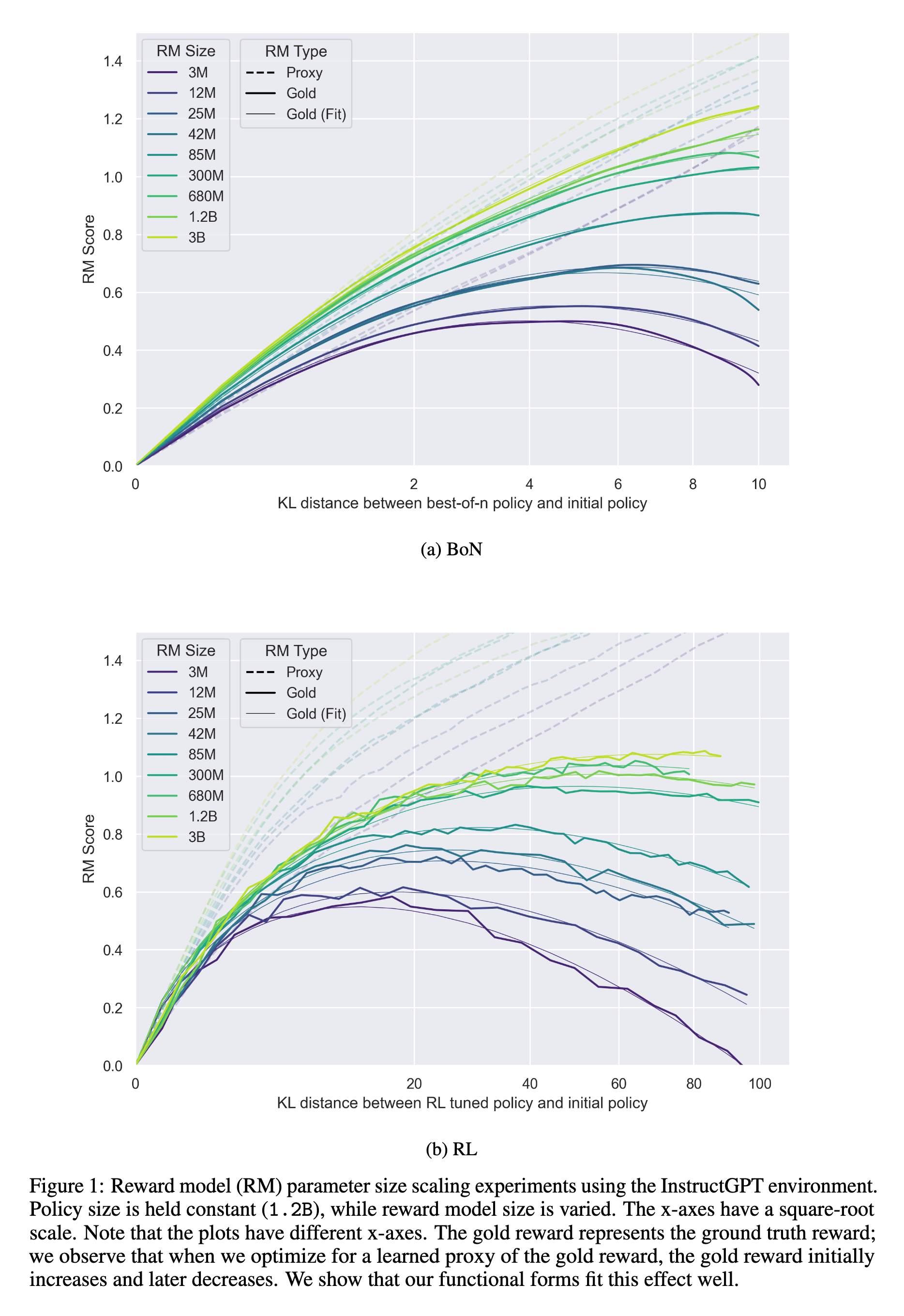
In the standard RLHF for LLMs, exploration is further constrained by a KL-divergence penalty. This penalty, $\beta \cdot \text{KL}(\pi_{\text{new}} | \pi_{\text{ref}})$, prevents the model ($\pi_{\text{new}}$) from drifting too far from its original distribution (typically the SFT or base LLM) ($\pi_{\text{ref}}$). This preserves language quality/fluency and prevents reward gaming, but it also constrains exploration by keeping the policy near its prior. KL-divergence can also be interpreted as a budget on policy deviation—a constraint that determines how far the model is allowed to move from its reference behavior during optimization. In this view, every training step “spends” part of this budget: increasing reward often comes at the cost of higher KL distance, meaning the model’s responses diverge more from its pre-trained tendencies. A small KL budget enforces conservative updates, maintaining linguistic fidelity but limiting potential reward gains. Conversely, a large KL budget allows greater policy flexibility and creative exploration, but risks linguistic degradation and reward hacking. Empirically, this trade-off forms a Pareto frontier between reward improvement and KL divergence, as shown in Scaling Laws for Reward Model Overoptimization (Gao, Schulman, Hilton, 2022). The x-axis represents KL divergence between the original and fine-tuned policies, while the y-axis shows the reward score. The curve demonstrates diminishing returns: beyond a certain KL threshold, additional divergence yields little reward gain and begins to degrade model alignment and quality.
In short: current post-training correction mechanisms are not enough. Exploration in RL-based fine-tuning for LLMs remains fundamentally insufficient—bounded by both policy entropy and KL regularization.
New Dimension of Exploration via Test-Time Compute
While RLHF and RLVR primarily regulate exploration during training through entropy and KL constraints, reasoning models unlock a new form of exploration at inference time. Rather than modifying policy weights, they extend the model’s capacity to search and evaluate alternatives within a single forward pass—through thinking tokens, multi-step reasoning, or deliberation loops.
This “test-time compute” serves as an orthogonal axis of exploration. Here exploration shifts from the policy space to the reasoning space: instead of sampling broader actions across training trajectories, the model explores deeper reasoning trajectories within each input. This shift mirrors classical ideas in decision-making systems, such as Monte Carlo Tree Search, where extra compute is spent exploring possible outcomes under a fixed policy. The difference is that LLM reasoning performs this exploration implicitly, through self-generated text that recursively conditions on its own prior thoughts. In this way, test-time compute effectively decouples exploration from the KL constraint. The model can maintain alignment and language quality by staying close to its post-trained policy distribution, while still exploring richer internal reasoning pathways.
However, unlike RL exploration, which receives explicit reward signals, test-time reasoning operates in a self-supervised vacuum. The model “explores” but doesn’t learn from it — it can’t improve future reasoning efficiency or correctness unless test-time reasoning is integrated into a training loop.
In short: test-time compute reframes exploration as a dynamic allocation of inference resources rather than parameter change. Yet without learning feedback, this form of exploration remains transient — capable of deeper thought, but not of lasting improvement.
Closing Thought
Can RL break the policy limits of pretraining? Partially.
Sutton’s view reminds us that intelligence is the capacity to act toward a goal. RL formalizes this pursuit through policies that maximize the reward. When extended to LLMs, this framework reveals both promise and constraints: pretraining and SFT teach imitation, while RLHF and RLVR introduce goal-directed correction but confines exploration within entropy and KL budgets. Test-time compute expands the picture by moving exploration from training to inference. Yet this new dimension of exploration exposes another issue: intelligence can search more deeply, but without feedback, it cannot learn from its own thought.
Recent reasoning-RL models (e.g., OpenAI o1, DeepSeek-R1, Gemini 2.5) couple RL with reasoning. Empirical evidence demonstrates initial success, e.g. Gemini “Deep Think” system recently reached a gold-medal standard at the International Mathematical Olympiad. Yet whether this paradigam can break the constraints from pretrained linguistic and semantic priors, discover genuinely new reasoning strategies rather than performing a fuzzy form of deduction, or induce the kind of creative abstraction that defines general intelligence.